Measuring Investment Performance

The Risk-Reward World

Investment is all about risk and return. Risk-averse investors want to maximise return for incurring a given level of risk or, put another way, minimise risk incurred for a given level of return. Everything gravitates around the risk-return trade-off, and professional investors and academics have devised ways of measuring this trade-off to separate the alpha that just a few can command from the beta that the market allows everybody to earn. But while it is relatively straightforward to measure return, the same cannot be said of risk measurement.

There are a few different ways of measuring return involving some degree of choice: discrete/continuous time, arithmetic/geometric means, normal/logarithmic scales, etc. But in the end, we can reasonably agree that, no matter the choice taken, return is the difference from end of period and beginning of period figures. When we move from return to risk, the case complicates, not least with regard to the definition of risk itself. A high degree of subjectivity is involved and a large number of choices and assumptions too. In the end risk is not measured as it should be and most of the time we both understate and overstate the real figure. Extreme returns are commonplace, capital draw-downs are frequent, and we end with crashes that no one seems able to explain.

Risk is often identified with volatility. If the average return represents the mean of the distribution, risk represents the variability of the return around that mean. Risk can be represented by a dispersion or variability measure; the standard deviation is often a good candidate. The larger the variability of each return observation around the mean return, the larger the standard deviation, and as far as risk is measured by the standard deviation, the larger the risk. But this is not something that is accepted by all, because it has strong assumptions behind it. When reality departs from those assumptions, real risk isn’t measured in a coherent way.

A Few Drawbacks with Risk Measures

Let me start with a very simple example with two pension plans, A and B, and a saver that wants to choose the plan that best preserves his purchasing power for retirement. Table 1 summarises the past performance achieved by the two pension plans.

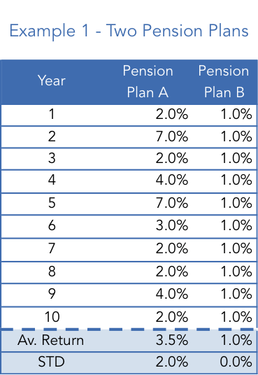
Plan A shows an average return of 3.5% while plan B averages just 1.0%. In a risk-neutral world (and provided that past performance is indicative of future performance for simplicity reasons), the saver would choose plan A. But the world is better described within a risk-averse framework and thus the choice is always two-fold requiring a comparison of return against some risk measure. The higher performance achieved by A comes with increased variability, as its standard deviation is 2% while for B it is 0%. If we accept standard deviation to be a good proxy for risk, plan B presents less risk, or no risk at all.

But we should never forget that the main goal of a pension plan isn’t to minimise the standard deviation of returns but rather to allow savers/investors to keep their purchasing power through time and thus retain their living standards upon retirement. Let’s suppose inflation averages 2% per year. While appearing less risky, pension plan B just failed to achieve its main goal and savers ended up losing purchasing power. The 1% average return falls short of the 2% average inflation rate.

While appearing riskier, plan B achieved its goals. One question that arises here is whether the likelihood of failure to achieve a given level of return represents a risk. If the answer is positive, then plan B must have some risk attached, as it failed to attain the required performance, but that risk is not captured by the standard deviation. We can also view the problem from the opposite perspective. If the main goal for a saver is to at least keep his purchasing power and since plan A has at least done that in each and every year, why would it be riskier than plan B? The standard deviation completely fails to answer this question. Just look at the numbers. Plan A returned at least 2% in every single year. The standard deviation captures the variability, which in plan A’s case has been the risk of performing above 2%. But, is that really a risk? The standard deviation penalises plan A for outperforming. Does it make any sense at all?

So, two drawbacks can easily be identified here: (1) the standard deviation doesn’t take into account the risk of failure to achieve some predefined level of return; and (2) it gives the same weighting to upside and downside deviations from the average. A fund that fails to meet its goals cannot be presented as zero risk and there is no such thing as upside risk (at least for long positions). A good risk measure should capture (1) as risk and (2) as no risk.

Measuring Performance

Now that we have some basic notions about risk and return and have identified a few drawbacks of standard deviation, let’s take a look at how we usually compare the performance of investments. We need to compute risk-adjusted returns such that the return of A is comparable with the return of B.

One of the most used measures is the Sharpe ratio or reward-to-volatility ratio. The measure is very simple to implement as it ranks funds, investments, and assets by the ratio of their excess returns to their standard deviation. It can be calculated as follows:

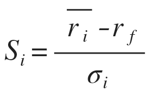
The average return for an investment i is computed. Then the return that can be obtained on a risk-free asset is subtracted from it (often the return on some government bond). Finally, this excess return is divided by the standard deviation of those returns. The Sharpe ratio shows the return per unit of total risk incurred. The higher the better.

Let’s now consider example 2 with Investments 1 & 2.

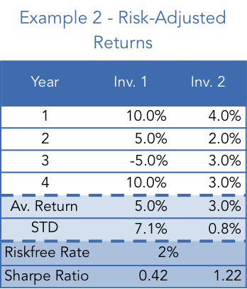
For the case in which the risk-free rate is equal to 2%, the Sharpe ratio for Investments 1 & 2 respectively is 0.42 and 1.22, which means Investment 2 ranks higher. While the average return achieved by 1 was superior, after adjusting for risk (as measured by the standard deviation), the reward per unit of risk is inferior. Under the Modern Portfolio Theory framework, one should always choose Investment 2, for which reward per unit of risk is higher.

Let’s say you have £100 and want to achieve a return of 5%. You can borrow £200 at 2% per year and then invest £300 in Investment 2. At the end of the year you will get a profit of £9 from Investment A (3% x £300) and you will have to pay £4 in interest (2% x £200). You end up with £5 on your €100, which is exactly 5%. The standard deviation of this portfolio is 3x the standard deviation of 2, which is 2.4 (because riskless assets have no associated risk). You just got the same performance as investment 1, but with much less risk. This is the basis of the Modern Portfolio Theory that explains why you should always invest in a well-diversified portfolio and get some leverage if you want to achieve higher returns.

The Sharpe Ratio Doesn’t Depict Reality

But while the Sharpe ratio is great when it comes to ranking assets, it does have some drawbacks. First of all, banks make money from the difference between the rate at which they lend and the rate at which they borrow. No one borrows at the riskless rate. In the above example you wouldn’t really borrow at 2%, which alters the picture a little. Another problem arises when returns are negative. Suppose both 1 & 2 offer a 5% return. For the stated standard deviation Sharpe ranks Investment 2 higher. But what would happen if the average return was -5% for both? Sharpe would rank 1 higher, even though it shows the same return as 2 on a larger standard deviation. The investment with higher risk would be ranked higher, which is against the main assumptions of a risk-averse world.

Apart from the two minor drawbacks outlined above, there are some bigger problems that are in part related with my comments at the beginning of this article. The standard deviation is a measure that assumes symmetry in the distribution of returns. It comes from the bell-shaped curve. For a mean return of 5%, both a 15% return and a -10% return are equally likely. It means that there must be no skew in the distribution. But we know there is a positive skew in equity returns as the market has an upward drift. At the same time some investment strategies are negatively skewed. In both cases there is an overestimate (first case) and an underestimate (second case) of risk when using the standard deviation. The bell-shaped curve also assumes there is no kurtosis, that is, investment returns have skinny tails. But that isn’t the case, as it has been documented over the years that extreme cases occur much more often than depicted in a bell-shaped curve (fat tails). The probability of an extreme case occurring (like a crash) is much higher than usually estimated when using standard deviation. The failure of the bell-curve to describe returns is therefore a problem.

Another issue is the fact that investors don’t distribute their concerns symmetrically around the average return. They distribute them asymmetrically, giving a large weighting to any negative deviations and no weighting at all to any positive deviations… and they don’t distribute such concerns around an average return but instead around a target minimum level of return they mentally conceive.

The Alternative Sort(ino)

Remember the pension plan case? Dispersions should be measured against the 2% required minimum target and not in turn of 3.5% or 1%. This would make plan B look much more riskier than before, as it would now show deviations in every single year. At the same time, because an investor is only concerned with negative misses, Investment 1 would now appear without risk, as it delivered at least the target return on every single year. When we think this way we are in Sortino’s world. The Sortino ratio does not consider the risk-free rate, instead replacing it for a target return, while also replacing the standard deviation by a partial standard deviation measure that takes into account the negative dispersions only. It can be calculated as follows:

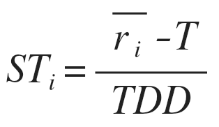
We can easily calculate the target downside deviation as follows:

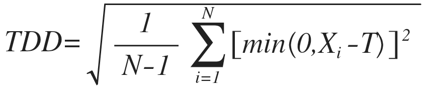
The target downside deviation is computed in a similar fashion as the standard deviation, but with two main differences. First of all, instead of a distribution mean, we now use the target rate T. Second, instead of considering all deviations, positive or negative, we now ignore all positive deviations (equal to zero or above).

Let’s now put Sortino into action and consider example 3a. We have two managers that have achieved a similar and fairly stable performance until the end of year 6. At the end of that year, the average performance was 2.8% and the standard deviation 1.6% for both. According to the Sharpe ratio they rank equally. Now comes year 7. Manager 1 achieves a huge 15% return while manager 2 can’t get more than 4%. At a glance, which manager would you choose?

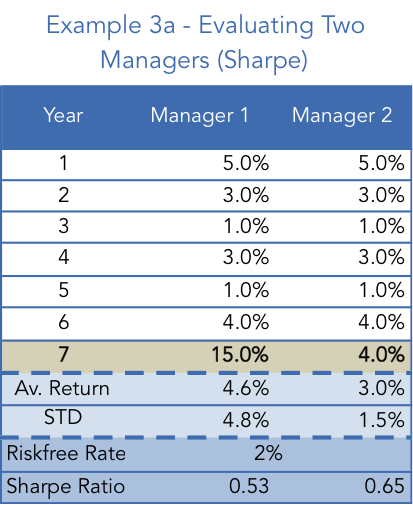
With both managers ranked equally at the end of year 6, and provided that manager 1 outperformed manager 2 in year 7, it seems natural to decide in favour of manager 1. But Sharpe’s measure would oppose such a decision, as it would rank manager 2 higher. The return obtained in year 7 increased the average return obtained by manager 1 but it also increased the standard deviation. But we know this increase was due to an outperformance and as such should be ignored and should not penalise A’s rank. Now for comparison reasons assume that the target rate for both managers is equal to the risk-free rate of 2%. Let’s take a look at what would happen when using the Sortino ratio instead.

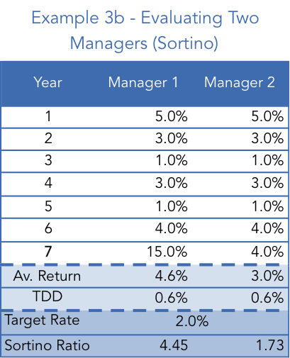
At the end of year 6 both would show a Sortino ratio of 1.44, but then with the return above the target rate both achieved in year 7 the ratio rises. As the deviation from the average on year 7 was positive no manager was penalised. Manager A then sees his Sortino ratio rise more than manager B. The Sortino ratio does a great job in capturing outperformance and disregards upside variability.

Some Final Words

In a world where returns don’t fit a bell-shaped curve and where upside variability isn’t an issue, one should take performance measures relying on standard deviation with a grain of salt. Upside and downside deviations aren’t equally likely and they aren’t equally undesirable. At the same time, an investor isn’t interested in the excess returns a fund can command over a riskless rate but rather in the excess returns it can command over some target rate. To overcome these difficulties, the Sortino ratio is a great tool.