The big flaw in Trump’s reflation plan

We have reached a point where people are so tired of the current economic model that they’re willing to support anyone promising to do away with the status quo and make life great again. It’s hard to find fault, because the current model is obviously rotten and is overwhelmingly biased towards the incumbent wealthy. But, with Trump now elected as President, things may change quite rapidly in terms of monetary policy, fiscal spending, and ultimately in terms of growth and inflation. Or so we’re told…

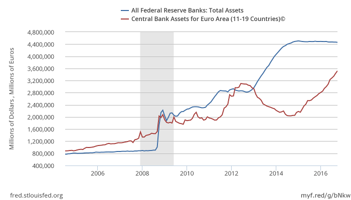
Until now, we have watched interest rates collapse and central bank assets soar. But such policy, mixed with fiscal tightening, has been relatively ineffective in terms of boosting growth to pre-crisis levels. Most of the positive effects have been lost in the translation from higher asset prices to higher growth, as the link between the financial economy and the real economy is clearly misunderstood by central banks. Explaining why central banks lost that link, what they can do to boost growth and how Trumpian fiscal spending may fare is my goal today.

Central banks’ missing link

Until the 1980s, central banks targeted monetary aggregates like M1, M2, M3 or some other measure of the money supply, because they relied heavily on the quantity theory of money, which predicts that an increase in the rate at which the money supply is growing will lead to a proportional increase in the inflation rate. Roughly speaking, if a central bank increases the money supply by 4%, it will induce a 4% increase in prices. Ergo, to keep inflation under control, the central bank needs to control the money supply.

We didn’t abandon the monetary aggregates, they abandoned us.

Until the 1980s, monetary targeting worked well around the world, but then central banks lost the link between the money supply and inflation and decided to abandon monetary targeting. The words uttered by Gerald Bouey, a former governor of the Bank of Canada, express the sentiment among central banks at the time: “We didn’t abandon the monetary aggregates, they abandoned us.”

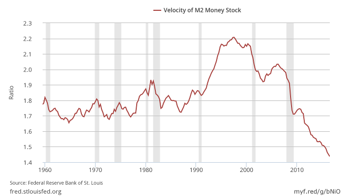
The classical theory in which monetary targeting was grounded stated that MV = PY (where M is the money supply, V is the velocity of money, P is the price level and Y the GDP). The velocity of money, which is an indication of money turnover, was expected to swing a little in the short term but to remain relatively unchanged in the long run, so some kind of mean reversion was always expected. But, suddenly, central banks lost the connection, as velocity started to decline in a continuous fashion. Under the traditional model MV = PY, it looked like the money was missing.

Unable to explain the connection between the real economy and monetary aggregates, academics found a very simple solution to the problem: they developed new models without money. The cashless New Keynesian models, which are the basis for modern central bank intervention, don’t link the real economy with the financial economy. This makes life easier for policy makers but is a major understatement of reality which may end with disastrous consequences. Banks are mostly out of the equation, which is the main reason why central banks weren’t able to predict their failure. Banks not only matter; they are the most crucial part of this system, as they have the ability to create money supply through credit, which is the main ingredient behind economic growth.


When Irving Fisher developed the original quantity theory, he stated that MV = PT (where T stands for transactions), which is a truism, an utterly obvious truth about the economy. The total amount of spending should always be equal to the total amount of money spent on those transactions. When we replace T for Y, we assume that T = Y (or at least, that T is a good proxy for Y). But we must always remember that T represents all transactions made during some time period, whether they relate to final products or financial assets. As Y represents GDP, it is a reduced form of T, excluding a significant group of transactions that are related to the financial economy. If I purchase shares in GSK, such a transaction is accounted for in T but not in Y.

An inevitable question arising here is: what if financial transactions start growing faster than GDP transactions?

Blowing bubbles

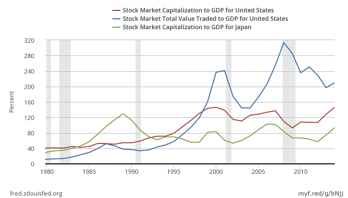
The U.S. equities market saw its capitalisation rise from 41.3% of GDP in 1980 to 146.3% in 2014, a 3.5x rise. Japan witnessed a similar trend – a rise from 30.6% to 93.7%. In terms of total value traded to GDP, the rise has been spectacular: in the U.S. the figure rose from 11.9% to 209.7%. One can only conclude that we have been witnessing a massive financialisation of the economy for the last 35 years. This must explain why central banks and academics lost the link proposed in the quantity theory. In using GDP, they’re missing a lot of transactions that are part of Fisher’s exchange equation. No wonder that velocity seems to be declining so rapidly.

While I don’t want to bore you with economic gibberish, I humbly ask for your patience in order to allow me to introduce here the work of an academic who explained the missing money link some 20 years ago – Richard Werner. (Those looking for further details can take a look at Werner (1997)* and Werner (2012)*.) Werner rightly claims that if we insist on using Y (GDP) to track the link to money, then we must add the missing part of the equation related to the non-GDP world of financial transactions. We can then split the original MV = PT into:

Vr x Mr = Pr x Y (where Vr is velocity associated to GDP transactions, Mr is money used for GDP transactions, Pr is a GDP deflator, and Y is GDP)

Vf x Mf = Pf x Tf (where Vf is velocity associated to financial transactions, Mf is money used for financial transactions, Pf represents asset prices, and Tf accounts for financial transactions)

where Vf and Vr are constant

and M  =  Mr + Mf

Through doing this, Werner is able to explain the puzzle of declining velocity. If most of the money goes into financial assets, then expect Pf x Tf to increase, not Pr x Y. But central banks don’t split transactions this way and thus, as they end up with Pr x Y mostly unchanged, they believe V to have declined. The response of central banks to this observed decline has been more asset purchases and negative rates, in order to force banks to lend more money and expand the money supply. That’s a deficient policy, as Werner helps us to understand. Central banks are expanding the money supply (M), but the most part goes to financial transactions (Mf expands much more than Mr). Changes in consumer prices and GDP are small because the change occurs mainly in the nominal value of financial transactions (Pf x Tf) instead.

Given that the cashless models of central banks don’t take account of the impact in the financial economy, they advise central banks to adopt additional unconventional policy measures. But through Werner’s lenses, we can see that central banks are just creating asset inflation. With ever bolder measures being adopted, the financial economy grows faster than the real economy, which in other words means an asset bubble is forming. Central banks miss the big picture and are responsible for the creation of asset bubbles and the corresponding boom and bust.


As with any bubble, at some point, credit conditions tighten. At that time, the positive feedback stops and the prices of financial assets decline. Banks cut back on all forms of credit, including credit for GDP transactions, which means that Mr will decrease. At this point we see spill-over from the financial economy to the real economy. Less credit for GDP transactions leads to a decline in nominal GDP, either through deflation, output declines or both. The central bank should at that point expand liquidity to banks, but make sure it is used to avoid the spill-over to the real economy and not to perpetuate the financial bubble. That may only be accomplished if the central bank distinguishes between credit to GDP and non-GDP transactions.

In 2007-2009 the FED should have provided liquidity to the real economy, not the financial economy. But, as it doesn’t make any distinction between the two, the S&P 500 has been hitting new highs while the real economy still lags behind. Hence the groundswell of support for Donald Trump.

Speaking of Trump, it’s time to look at the hope he brings to the real economy. He is right about the massive distortions central banks are delivering.

Will the Trumpian fiscal shock work?

According to Werner, the only way to increase nominal GDP (Pr x Y) is by increasing the money attached to these transactions (Vr x Mr). That means increasing credit to the real economy. If monetary conditions are tightened, as Trump wants and Yellen seems to be willing to deliver, his fiscal spending drive won’t work. Any attempt to increase government spending will be fully reversed by a decline in consumption, investment and net exports if not accompanied by credit expansion. As Werner explains, in order to boost the economy, the government can’t issue bonds, it must borrow from banks. When issuing bonds, the government is just replacing one type of spending by another, which isn’t really expansionary. When borrowing from banks, the government is forcing banks to expand credit to GDP items. That’s the key to unlocking growth potential, as depicted in Werner’s equations!

If monetary conditions are tightened, as Trump wants and Yellen seems to be willing to deliver, his fiscal spending drive won’t work.

Finally, a few words on the banking crisis and the bailout system adopted in Europe. As predicted above, to avoid a spill-over from the financial economy to the real economy, governments should borrow from banks. What happened in Europe? Banks borrowed from governments. If the first is expansionary, the second must be contractionary, which explains the huge contraction experienced in Europe.

To conclude, central banks got it all wrong. Monetary policy is being conducted pro-cyclically and central banks are to blame for boom and bust. Explaining the economy with a cashless model is like explaining the equity market without any reference to equity prices.

* Werner (1997) – Towards a New Monetary Paradigm: A Quantity Theorem of Disaggregated Credit, with Evidence from Japan; Kredit und Kapital 2(2), pp 276-309.

* Werner (2012) – Towards a New Research Programme on ‘Banking and the Economy’ — Implications of the Quantity Theory of Credit for the Prevention and Resolution of Banking and Debt Crises; International Review of Financial Analysis 25, pp 1-17.