Why Is There No Inflation (And No Growth)?

One of the most puzzling questions central bankers have been asking themselves during the last few years is: why is inflation so low when the money supply has expanded so much? At the same time, and after realising it, then comes a second question: with inflation being so low, why isn’t growth much higher at a time the money supply has expanded so much?

Traditional monetarist wisdom claims that the growth in the money supply should be roughly equal to the growth in prices less the growth in GDP. But when such theory is applied to the U.S. economy it seems to fail. Between 2008 and 2013, the money supply grew at an average of 33% per year while inflation grew at an average of 2%. For the monetarist view to be right, GDP growth should have averaged 31%. This observation has been the base for the WSJ criticism of the Fed’s QE, as not being able to boost GDP. But then one can think in a different direction. Between 2008 and 2013, the money supply grew at an average of 33% per year while GDP averaged 2%. For the same view to hold, inflation should have averaged 31% per year. This observation led to the counter-attack from Ben Bernanke blaming the WSJ for forecasting a breakout in inflation and a collapse in the dollar at least since 2006. Who is right? What is happening here? Is the Quantitative Theory dead?

A Misspecification

Over the years, several errors have been committed in the formulation of monetary policy, in the individual decision making, and in the understanding of the current reality, which leads to aberrant conclusions that are just based on wrongly formed assumptions and distortions of theory. The above situation is an example of how the original Quantity Theory of Money has been abused and, as a consequence, led to wrong claims. Apart the reciprocal blames exchanged between the former Fed chairman and the WSJ editorial, others have preferred to claim the velocity of money is not as it used to be. It must have decreased as a result of people hoarding money, which explains why GDP and inflation are both low. This observation additionally supports the view that the money supply needs a very large boost in order to impart the expected effects and that monetary policy should adopt extreme measures. Such a view takes the monetary policy to a military level where instead of fine tuning we speak of bazookas and other kinds of artillery.

All this is a tremendous misunderstanding and misspecification of the Equation of Exchange, presented by Irving Fisher in 1911, which gave rise to the Quantity Theory of Money.

The Equation of Exchange (which is an identity and not really an equation) is relatively simple to understand. It is usually expressed as:

(1) MV = PT

What the equation claims is that the quantity of money available in a certain period times the velocity at which each unit is on average spent should be equal to the total number of transactions made in the same period times an average price level. The total expenditure or money spent (MV) should be equal to what is purchased with that money (PT). That must be absolutely true. The velocity of money was assumed to be constant, such that the rate of increase in the money supply should be equal to the rate of increase in prices less the growth in transactions. In the long run, if V and T grow at the same pace, inflation would be essentially a monetary phenomenon and any attempt to increase the money supply would translate into proportional price rises.

But then economists were not happy with this identity and rewrote it in a way to make it workable. Then comes:

(2) MV = Py

Py is not anything more than nominal GDP and it is now easily measured. But, it is not in accordance with Fisher’s identity. GDP ignores the fact that the same product may be resold several times in a certain time period. It also ignores products that were produced before that time period even if they were sold within it. GDP only accounts for newly produced goods and services, while T measures all transactions including those on pre-existing assets like financial assets and property.

In summary, economists weren’t able to measure T, so they found a proxy for it. Real GDP was the closer proxy, so the problem seemed solved. At the same time, it is tough to measure money, so a monetary aggregate is usually used as proxy for M. But then, we are no longer sure about the result deriving from this formula, and thus we don’t really know what a decrease in the velocity of money really means.

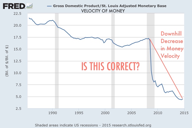
If we use the St. Louis Adjusted Monetary Base as a proxy for the money supply (as it is often used, just check here for example) and nominal GDP as a proxy for Py, then we have the confirmation of a quick decline in the velocity of money.

In particular, since 2007 the velocity of money has been on a downhill race.

Such findings would be absolutely stunning were it not for the fact that the proxies used are quite a distortion of the original Equation of Exchange.

Transactions on Amazon shares and on property are ignored. There’s no counterpart on the right hand side of the equation (2) for some of the money that changed hands on the left side of it. So the only way for V to capture this missing link is by decreasing. In that sense, the observed decrease in V may just be a consequence of misspecification.

But let’s now pretend that GDP is a good proxy for transactions. Is the monetary base the same as money or money supply? What really is money? Money is the total amount that left some hands during a time period in exchange for the real and financial assets that left other hands. In a fractional reserve system, where commercial banks expand base money several times through credit creation, we should take the St. Louis Monetary Base as money only with a grain of salt. M0 is not money, it is just a small and variable fraction of what serves as money. Money would be better measured with some broad credit measure instead, or at least using M1 (even though there’s no guarantee that M1 corresponds to the total money used in transactions).

The above chart doesn’t measure the velocity of money but rather the velocity of the monetary base, and assumes that money can’t buy non-GDP items. But it is often used as proof that the velocity of money has been decreasing. The explanation then comes naturally as: “individuals are hoarding cash”; and the prescription as: “we must make them spend it”.

The Missing Link Between Real and Financial Items

What I told you in the beginning of this article is not quite correct. I said the money supply expanded at an average of 33% per year during the period 2008-2013. But that is what is said by the Assistant VP and a Research Assistant of the Fed of St. Louis in their explanation for the decline in the velocity of money. But they use the monetary base and nominal GDP, which are bad proxies for our relation. Let’s see why.

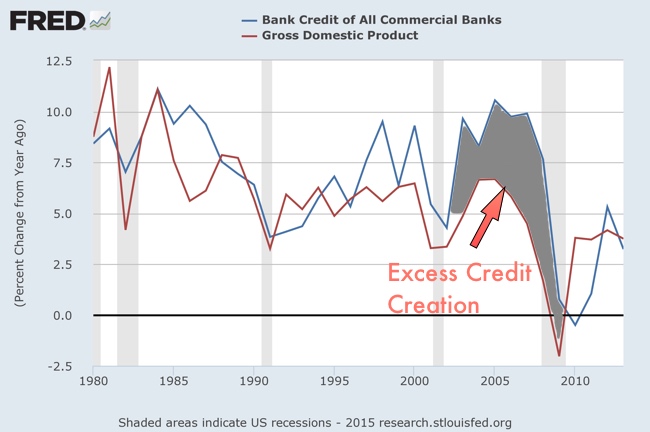
Prof. Richard Werner from the University of Southampton developed an alternative theory (1992, 1997, 2005) – the Quantity Theory of Credit, which in my opinion helps explain the missing link between the original Equation of Exchange and the recent empirical evidence. He claims that the best proxy to measure the money supply is credit. In a fiat money system we should look at credit as a proxy for what was really spent and never at a monetary aggregate. There’s no connection between M0 and credit, as the mainstream money multiplier model doesn’t hold. Banks create as much credit as they want and that credit is what serves as money in transactions, not the central bank reserves. M1 would better reflect credit as it includes deposits but we’re not sure part of that money isn’t just parked at banks. So, M should be proxied with some variable measuring credit.

But the most important part of Werner’s theory comes from the recognition that money may be spent on non-GDP items like Amazon shares and property. He reformulates the Equation of Exchange in two separate equations reflecting the real economy (3) and the financial economy (4):

(3) M(r) V(r) = P(r) y

(4) M(f) V(f) = P(f) T(f)

and finally (5) M = M(r) + M(f)

The money supply, proxied by total credit given by commercial banks, can be spent in the real economy in the form of investment or consumption (equation 3) or in the financial economy to buy pre-existing assets like shares or property (equation 4). This redefinition goes a long way in explaining the missing link that everybody fails to understand. During boom times, no one perceives any risk. Optimism rises and banks expand credit. The majority of the created money is spent in the financial economy, acquiring property and financial assets. Prices then rise pushing optimism even higher and, with it, the willingness of banks to offer further credit.

Of course this credit will end mostly spent in financial assets again. Believe it or not, credit for investment activities is a ridiculously small part of total credit (in most countries, including the UK), so most of the credit is not spent in expanding output capacity.

If credit goes to investment, then y in the equation (3) expands with M(r) and such expansion is non-inflationary. If credit goes to consumption, it doesn’t push y higher and thus is inflationary.

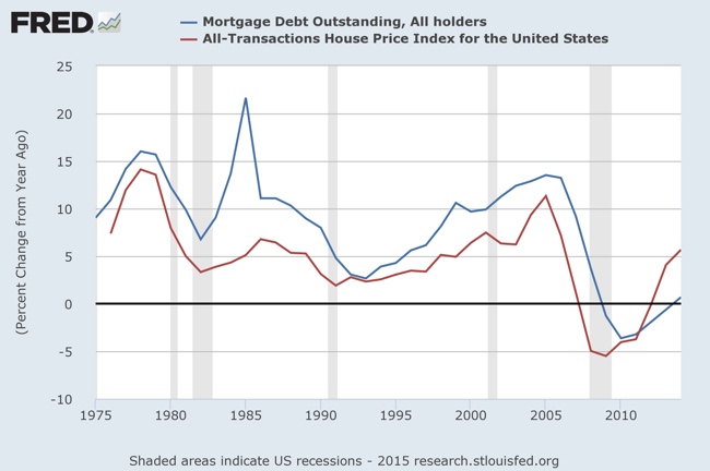
But as I mentioned above, money is mostly spent to acquire pre-existing assets. Just think about what happened before the financial crisis of 2007-2009. Most of the expansion in the money supply went directly to the property market, which accordingly to the Werner’s specification doesn’t generate consumer inflation but rather asset inflation. This is because this market has a relatively inelastic supply (a characteristic also shared by financial assets). That means that T(f) in equation (4) is more or less constant. That being true, when banks expand credit too much, most of that expansion leads to an increase in M(f) and not in M(r). As a consequence and because T(f) is relatively rigid, asset prices rise and bubbles form. The connection between house prices and credit to purchase them is very strong.

During such credit booms there’s no reason to expect CPI to rise, in particular in economies heavily dependent on non-GDP items. This is a strong clue as to the missing link between the expansion of the money supply and a rise in CPI.

One could say that, later on, higher asset prices should translate into increased perceived wealth and then spill over to the real economy through increased consumption. That may be the case and consumer inflation may by then start rising. But at that time central banks start increasing their interest rates and tightening policy and the initial optimism vanishes.

Why is there consumer deflation?

When the optimism vanishes banks start realising that a large part of their loans will never be repaid. By then they cut credit by as much as possible. The deleveraging process starts and everybody tries to pay down debt. To counterbalance such a deflationary scenario, the central bank adopts unconventional measures to spur the money supply, by purchasing assets directly. As we have seen recently, such policy puts a floor on asset price deflation, preventing a downward spiral in asset prices. But is it really effective in expanding the money supply available for real purchases? No, it isn’t.

Banks contract all credit (for real and financial purposes) and the central bank policy is unable to discriminate between the real and financial economy. Unless the central bank directly finances government spending (and supposing such spending is directed towards investment activities), there’s no way to discriminate and direct funds towards investment through financial asset purchases. This explains why inflation remained subdued while GDP was growing less than mildly over the last few years. That’s because the expansion of M has been mostly due to an expansion of M(f) rather than M(r). The financial economy is the part capturing the inflation, not the real economy. This explains why Ben Bernanke wasn’t able to spur economic growth during his second mandate and why the WSJ editorial’s predictions on inflation didn’t materialise. Additionally it predicts that we are heading towards another financial bubble.

A Few Final Words

While I still believe the current fractional system is part of the problem rather than the solution, because money creation is at the discretion of commercial banks (for a further development on the subject read my article in the next issue of Master Investor Magazine), one thing becomes clear in Werner’s exposition: it doesn’t just matter how much credit is being created but also (and foremost) where it is going to be spent.

If the additional credit is spent in the relatively inelastic financial economy, then we must expect asset price bubbles and banking crises to repeat every X years. If the additional credit goes towards the real economy, then we must still be careful with its direction. Credit for consumption is often inflationary while credit for investment creates growth and is not inflationary. With the above in mind, if we follow a model with government/central bank intervention, then we should at least do it right. It is not a matter of buying, but a matter of buying the right things, with those being the inputs that allow output expansion and growing economic wealth.

The rationale behind all this is quite simple. Just forget about any maths and the equations depicted above and think about the economy. When we purchase things with money, we are in fact exchanging two products (as the money we hold is the payment we received for our effort to produce other goods and services, in the form of labour). The transaction ends with the exchange. But now replace money with credit. When credit is expanding in the economy, more and more purchases are being tied to future wealth. The more the credit expands, the greater the future wealth that is required to repay it. Suppose that such purchases are not directed towards investment. Then future wealth will remain constant. How can then credit ever be repaid? It can’t and it never will.

It’s time to think about all these issues properly before we destroy the future of our kids. We either prevent banks from expanding credit or redirect that credit to investment purposes.